The Koch snowflake fractal has another interesting property common to fractals in that it has a 'fractal dimension'. Lines have dimension 1, squares have dimension 2, and cubes have dimension 3, but the limiting Koch function has dimension approximately 1.2618, a dimension higher than that of a line(1), but less than that of a square(2), since the figure does not fill the plane.
If a self-similar figure contains n copies of itself and each copy has length s, then the fractal dimension D is defined to be ln(n)/ln(1/s). In this case each segment contains 4 copies of itself and each copy is 1/3 as long as the previous length.
So D = ln(4)/ln(1(1/3)) = ln(4)/ln(3)= 1.2618595071429148
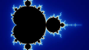
You can see an interactive version of the Mandelbrot set here.
In this interactive version you can see for yourself the self-similarity property by clicking on this graph with the left button of the mouse, then dragging the mouse a short distance away and releasing. You will then see the small section you have chosen enlarged to fill the graph.
You can also see the complexity in the following two YouTube videos which zoom into the Mandelbrot set to a great depth.
Note in this video the recurring Mandelbrot sets which appear as it zooms in further and further.
In this video the final area is covers a very small fraction of the area of the beginning area (about 1/10^72 = 0.000...0001 with 72 zeroes in that number.) Even deeper levels can be computed, but there are limitations with the size of the numbers the computer can manipulate.
These seemingly chaotic graphs are formed by a very simple mathematical process. Go to the mathematics link for a short description of the mathematics behind the Mandelbrot set.
You can see an interactive version of the Julia Set here. Again you can show the self-similarity by dragging a rectangle across any section of the graph you wish to enlarge.
Some examples are shown in the following
video which demonstrates some of these Julia sets. The various constants used are points from the Mandelbrot set.
Every point which converges by this method to z=1 will be colored red. The points which converge to the other two complex sroots will be colored green and blue respectively. This will create three basins of attraction in the three colors. Again, you can see the self-similarity by dragging a rectangle and clicking the Redraw button.
Some of the mathematics of this technique may be further studied in
Example 2
of the link to a website on chaos.
Iterated Function Systems are used to form some pictures like the Sierpinski triangle, which is created by applying a set of three functions, or transformations, to the points contained in a triangle.
The mathematics of the creation of a Sierpinski triangle by an Iterated Function System can be further examined at this link.
Another example is a set of four functions, which when iterated, yields the Barnsley fern.

The following video zooms into the Barnsley fern to show the self-similarity-i.e.-each leaf is similar to the whole fern and each branch on each leaf is also similar to the whole fern.
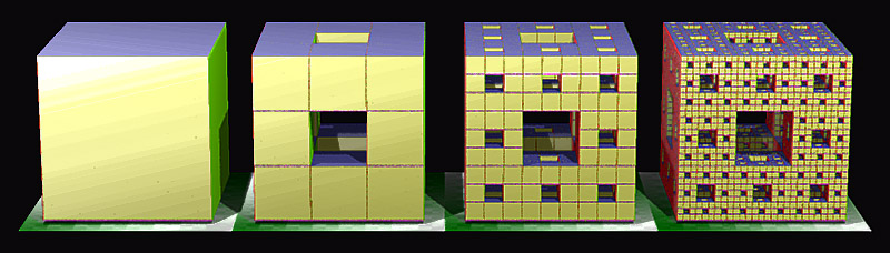
Iterated Function Systems can be used to produce other fractals as well, such as the 3 dimensional Menger sponge.
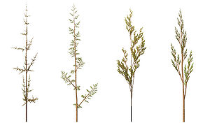
Some rather realistic plants can be drawn with L-Systems, such as the 'weeds' below:
The mathematics of this technique may be further studied in Example 1 of the link to a website on chaos.